Deep Learning for Photonic Structure Design

(Jan. 2024 - Jul. 2024)
Introducing a faster and more convient way in doing Photonic Structure Design.
Introduction
As deep learning has developed over the years, it has been used in many different fields to help workers increase efficiency. Our team, under the Shcherbakov Nanophotonics Lab, led by PhD researcher Melika Momenzadeh, is working towards using deep learning to find the best parameters for a photonic structure that lead to the highest possible transmission rate.
Our 4-input Forward Deep Learning Design
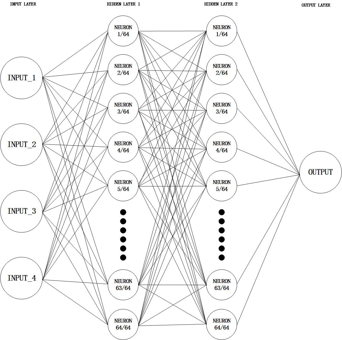
In this part, I developed a neural network model for forward design using TensorFlow and Keras. The dataset I used contains 1,500,000 sets of data. Each set has 4 inputs and 1 output and I utilized NumPy and Pandas for efficient data handling.
Model Architecture:
- Input Layer: Adjusted to match the shape of the training data.
- Hidden Layers: Two dense layers with 64 neurons each and ReLU activation functions to capture complex patterns in the data.
- Output Layer: A single neuron with a linear activation function for regression tasks.
Model Training:
- Compiled the model with the Adam optimizer and Mean Squared Error loss function.
- Implemented early stopping to prevent overfitting by monitoring validation loss and restoring the best model weights.
Results:
The graph below illustrates the training and validation loss over the epochs. The rapid decrease in loss indicates that the model effectively learned from the data, achieving a low error rate.
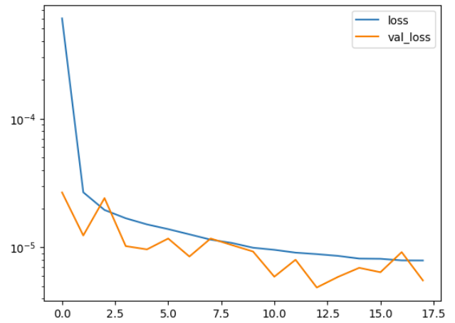
Additionally, the model's prediction accuracy was tested on new input data. For instance, given the input features [5.90003e-06, 2.11111e-07, 3.88889e-07, 4.77778e-07], the model predicted a value of 0.9025833, closely matching the expected value of 0.903052.

Our 52-input Forward Deep Learning Design
After completing the 4-input forward design, we increased the complexity of the project by adding more inputs, representing additional parameters of a photonic structure, into the dataset. For the following model, I trained it using a dataset containing 15,510 data sets.
Data Loading and Preprocessing:
- Data was also loaded using Pandas to handle irregular spaces.
- Identified and handled rows with NaN or infinite values by either removing them or replacing them with the mean of the respective column.
- Split the cleaned data into training and testing sets using
train_test_splitfrom Scikit-Learn. - Standardized the input features with
StandardScalerto ensure consistent model performance.
Model Architecture:
- Input Layer: Adjusted to match the shape of the training data.
- Multiple Dense Layers: Layers with 1024, 512, 256, and 128 neurons, each followed by BatchNormalization and Dropout for regularization.
- L2 Regularization: Applied to each dense layer to prevent overfitting.
- Output Layer: A single neuron with a linear activation function for regression tasks.
Model Training:
- Compiled the model with the Adam optimizer and Mean Squared Error loss function.
- Implemented a learning rate scheduler to adjust the learning rate dynamically during training.
- Early stopping and learning rate reduction on plateau callbacks were used to enhance training efficiency and model performance.
Results:
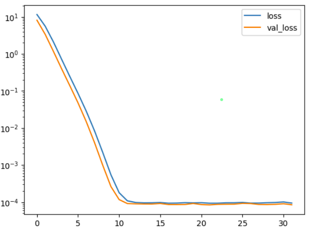
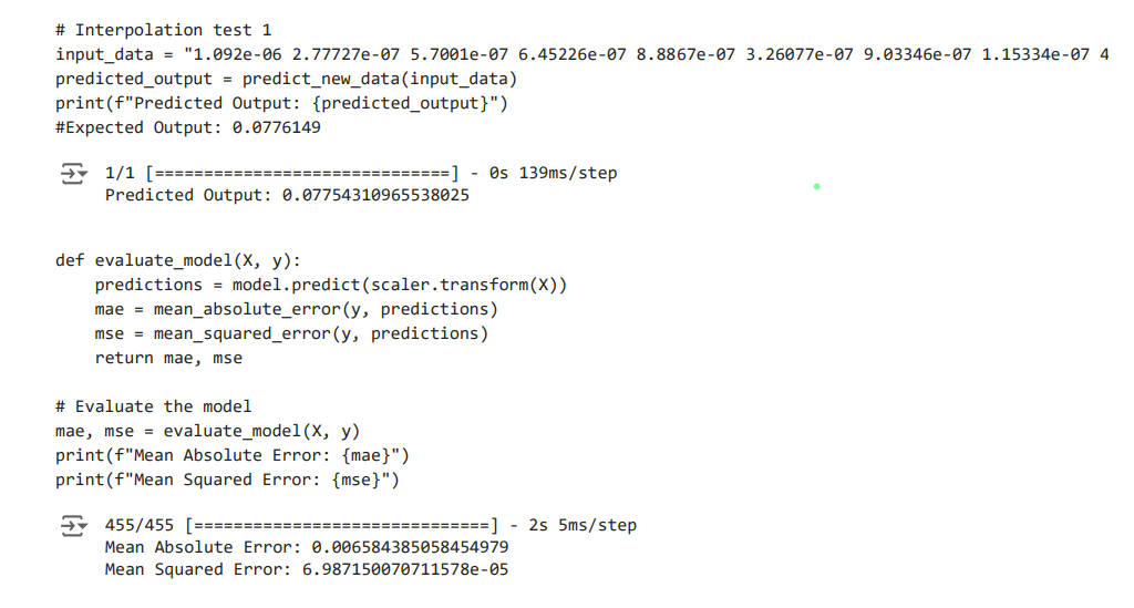
The first image displays a graph showing the training and validation loss over epochs; The second image displays a portion of the code and the corresponding outputs for model prediction and evaluation.
- Mean Absolute Error (MAE):
0.006584385058454979, indicating the average magnitude of errors between the predicted and actual values. - Mean Squared Error (MSE):
6.987150070711578e-05, indicating the average squared difference between the predicted and actual values.
Inverse Design Models
As of now, the team is moving on to work on inverse designs of the neural network models we have trained. This means that we want to input a transmission rate, and the model will tell us the exact parameters of a photonic structure, allowing us to create better structures more efficiently.
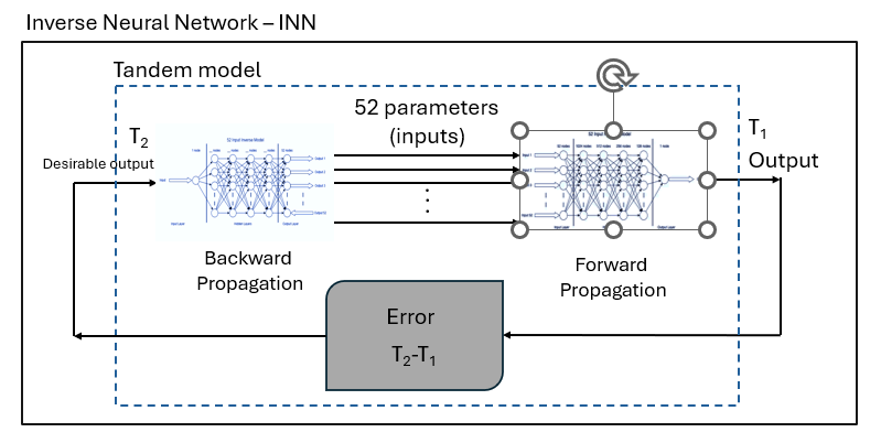
Tandem Model:
The tandem model was the first one we tried. This model uses iterative methods to create an inverse neural network model. The problem with this model is that it performs poorly with extrapolation data, and extrapolation prediction is essential for our project.
cVAE Model:
A Conditional Variational Autoencoder (cVAE) is a type of neural network designed for generating data conditioned on a specific input. It extends the traditional Variational Autoencoder (VAE) by incorporating labels or other conditional information into both the encoder and decoder networks, enabling more controlled and targeted data generation. Although cVAEs struggle with extrapolation data input, their powerful structure can potentially help increase the accuracy of many of our current models. The following explains the basic structure of the model.
Sampling Layer:
- A custom
Samplinglayer is defined for the cVAE, which generates random samples from the latent space during training. This is essential for the reparameterization trick used in VAEs.

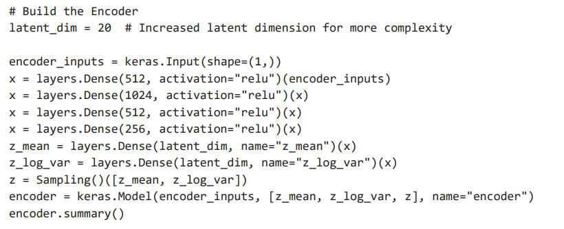
Encoder Architecture:
- The encoder takes the transmission value as input and passes it through multiple dense layers with ReLU activation functions.
- The encoder outputs the mean and log variance of the latent space, along with the sampled latent vector.
Decoder Architecture:
- The decoder takes the latent vector as input and reconstructs the design parameters through multiple dense layers with ReLU activation functions.
- The output layer uses the softplus activation function to ensure non-negative design parameters.

Special Thanks
Dr. Maxim Shcherbakov – – Head of the Shcherbakov Nanophotonics Lab – – maxim.shcherbakov@uci.edu
Melika Momenzadeh – – Head of the project – – mmomenza@uci.edu
Kiril Afonchenko – – Student Researcher – – kafonche@uci.edu
Tangqin Zhu – – Student Researcher – – tangqinz@uci.edu
Samuel Glushkin – – Student Researcher – – sglushki@uci.edu
Massee Akbar – – Student Researcher – – akbarms@uci.edu
Sam – – Student Researcher – – illarionova.23@uwc-usa.org